Editor's note: DRDO researcher Ayoosh Kathuria discussed in depth how the activation function implicitly changes the distribution of data passed into the network layer, thereby affecting the optimization process of the network.
This is the third article in the optimization series. We want to review the optimization techniques in deep learning through this series of articles. So far, we have discussed:
Mini batch gradient descent for combating local minima and saddle points
Momentum, RMSProp, Adam and other methods have strengthened on the basis of the original gradient descent to deal with the problem of ill-conditioned curvature.
Distribution, damn distribution, and statistics
Unlike previous machine learning methods, neural networks do not rely on any probabilistic or statistical assumptions about the input data. However, in order to ensure that the neural network learns well, one of the most important factors is that the data passed into the neural network layer needs to have specific properties.
The data distribution should be zero centered, that is, the mean of the distribution should be near zero. Data that does not have this property may cause gradients to disappear and training jitter.
The distribution is best to be normal, otherwise it may cause the network to overfit a certain area of ​​the input space.
During the training process, the activation distributions of different batches and different network layers should be kept consistent to a certain extent. If this property is not available, then we say that the distribution has an internal covariate shift (Internal Covariate shift), which may slow down the training process.
This article will discuss how to use activation functions to deal with the first two problems. At the end of the article, some suggestions for choosing the activation function will be given.
Vanishing gradient
The vanishing gradient problem has a wealth of documents, and as the neural network gets deeper and deeper, this problem is getting more and more attention. Below we will explain why the gradient disappears. Let us imagine the simplest neural network, a set of linearly stacked neurons.
In fact, the above network can easily be extended to a deeply densely connected architecture. Just replace each neuron in the network with a fully connected layer using the sigmoid activation function.

The image of the sigmoid function looks like this.
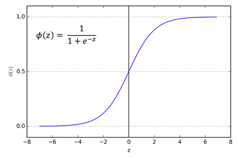
Looking at the slope of the sigmoid function, we will find that it tends to zero at both ends. The sigmoid function gradient image can confirm this.
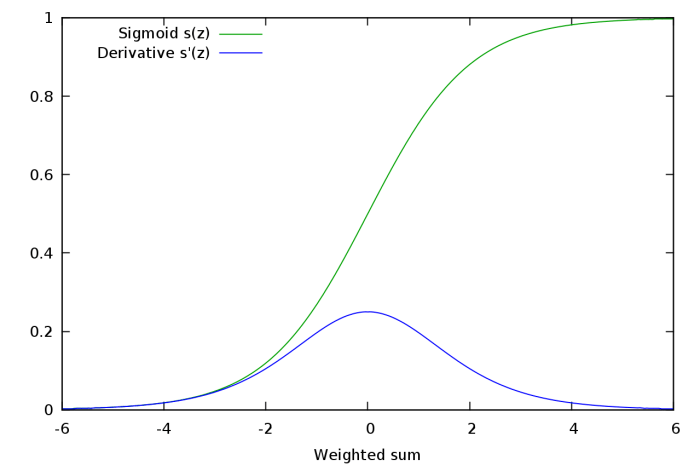
When calculating the derivative of the output of the sigmoid activation layer on its weight, we can see that the gradient of the sigmoid function is a factor in the expression, and the value of the gradient ranges from 0 to 1.

The second term in the above formula is the derivative of sigmoid, with a value range of 0 to 1.
Going back to our example, let's find the gradient of neuron A. Applying the chain rule, we get:

Each term in the above expression can be further decomposed into the product of gradients, one of which is the gradient of the sigmoid function. E.g:

Now, suppose that there were not only 3 neurons before A, but 50 neurons. In practice, this is completely possible, and the network in practical applications can easily reach 50 layers.
Then the gradient expression of A contains the product of 50 sigmoid gradients, and the value of each term ranges from 0 to 1, which may push the gradient of A to zero.
Let us do a simple experiment. Randomly sample 50 numbers between 0 and 1, and then multiply them.
import random
from functools import reduce
li = [random.uniform(0,1) for x in range(50)
print(reduce(lambda x,y: x*y, li))
You can try it yourself. I tried many times, and I never got a number of magnitude greater than 10-18. If this value is a factor in the gradient expression of neuron A, then the gradient is almost equal to zero. This means that in the deeper architecture, the deeper neurons basically do not learn, even if they learn, the learning rate is extremely low compared to the neurons in the shallower network layer.
This phenomenon is the problem of vanishing gradients. The gradient in deeper neurons becomes zero, or in other words, disappears. This leads to extremely slow learning of the deeper layers in the neural network, or, in the worst case, no learning at all.
Saturated neuron
Saturating neurons will further exacerbate the vanishing gradient problem. Suppose that the pre-activation value ωTx + b of afferent neurons with sigmoid activation is very high or very low. Then, since the gradient of the sigmoid at both ends is almost 0, any gradient update basically cannot cause the weight ω and the bias b to change, and the weight change of the neuron takes many steps to occur. In other words, even if the gradient is not low originally, due to the existence of saturated neurons, the final gradient will still tend to zero.
ReLU savior
Under ordinary deep network settings, the introduction of the ReLU activation function is the first attempt to alleviate the problem of gradient disappearance (LSTM is also introduced to deal with this problem, but its application scenario is a cyclic model).
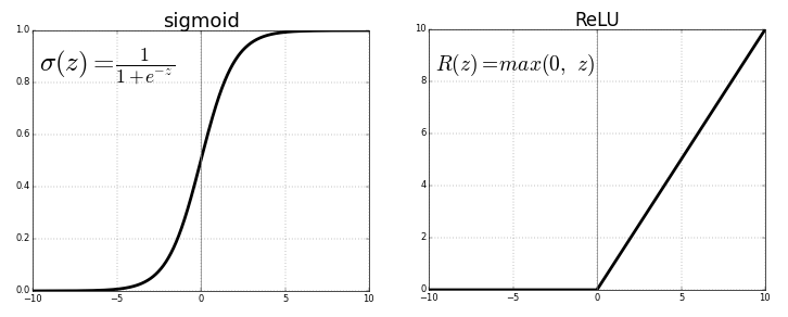
When x> 0, the gradient of ReLU is 1, x
Unilateral saturation
The sigmoid function is bilaterally saturated, that is, both the positive and negative directions tend to zero. ReLU provides unilateral saturation.
To be precise, the left half of ReLU is not called saturation. In the case of saturation, the function value changes very little, while the left half of ReLU does not change at all. But the roles of the two are similar. You may ask, what are the benefits of unilateral saturation?
We can think of neurons in a deep network as switches, which are specifically responsible for detecting specific features. These characteristics are often called concepts. The neurons in the high-level network may eventually specifically detect high-level features such as eyes and tires, while the neurons in the low-level network will eventually specifically detect low-level features such as curves and edges.
When such a concept exists in the input of a neural network, we want to activate the corresponding neuron, and the magnitude of activation can measure the degree of the concept. For example, if a neuron detects an edge, its magnitude may indicate how sharp the edge is.

However, the negative value of the neuron is meaningless here. It feels weird to use negative values ​​to encode non-existent concepts.
Taking a neuron that detects edges as an example, a neuron with an activation value of 10 may detect a sharper edge compared to a neuron with an activation value of 5. But it doesn't make much sense to distinguish neurons with activation values ​​of -5 and -10, because a negative value means that there is no edge at all. Therefore, it is very convenient to uniformly use zero to indicate that the concept does not exist. The unilateral saturation of ReLU fits this point.
Information unwrapping and robustness to noise
Unilateral saturation improves the robustness of neurons to noise. why? Assume that the value of the neuron is unbounded, that is, it is not saturated in both directions. Inputs with different degrees of concepts produce different positive outputs of neurons. Since we want to indicate the strength of the signal in orders of magnitude, this is good.
However, background noise and concepts that neurons are not good at detecting (for example, the area containing the arc is passed into the neuron that detects the line), which will generate different negative output of the neuron. Such differences may bring a lot of irrelevant and useless information to other neurons. This may also lead to inter-unit correlation. For example, neurons that detect lines may be negatively correlated with neurons that detect arcs.
In the scenario of unilateral neuron saturation (negative), the difference caused by noise, that is, the magnitude of the previous negative output, is squeezed to zero by the saturation element of the activation function, thereby preventing the noise from generating irrelevant signals.
Sparsity
The ReLU function also has advantages in computing power. ReLU-based networks are faster to train, because calculating the gradient of ReLU activation does not require much computing power, while sigmoid gradient calculation requires exponential calculations.
ReLU is reset to the negative value before activation, which implicitly introduces sparsity to the network and also saves computing power.
Death ReLU problem
ReLU is also flawed. Although sparsity has advantages in computing power, too much sparsity can actually hinder learning. The neuron before activation usually also contains a bias term, if the bias term is a too small negative number, so that ωTx + b
If the learned weights and biases make the pre-activation values ​​of the entire input field negative, then the neuron cannot learn, causing a saturation phenomenon similar to sigmoid. This is called the death ReLU problem.
Zero centralized activation
Regardless of the input, ReLU only outputs non-negative activations. This may be a disadvantage.
For a neural network based on ReLU, the activation of the weight ωn of the network layer ln is

Therefore, for the loss function L:

The I in the above formula is an indicator function. When the incoming ReLU value is positive, it outputs 1; otherwise, it outputs 0. Since ReLU only outputs non-negative values, the positive and negative gradient updates of each weight in ωn are the same.
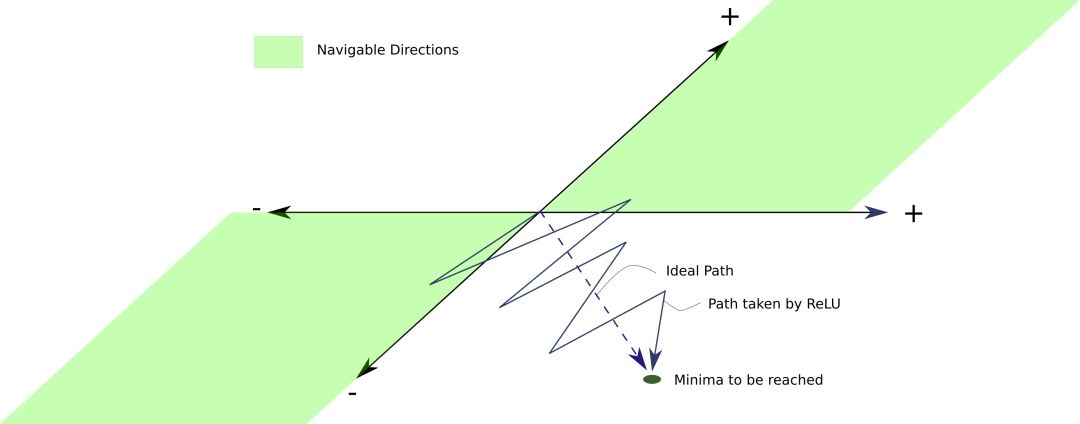
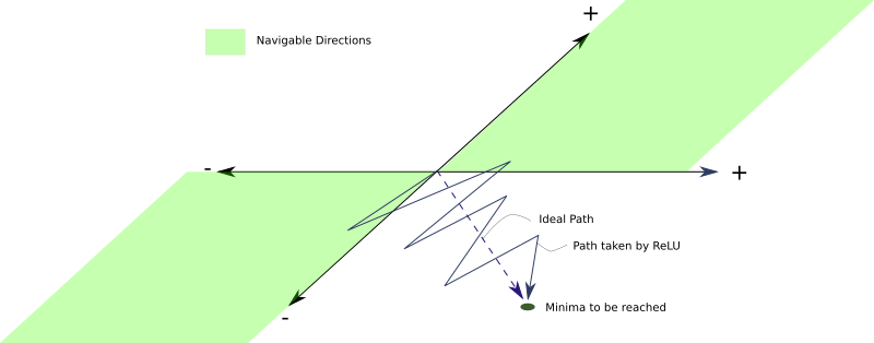
What's wrong with this? The problem is that since the signs of the gradient update of all neurons are the same, all the weights in the network layer ln will either all increase or all decrease in one update. However, an ideal gradient weight update may be that some weights increase and some weights decrease. Under ReLU, this can't be done.
Suppose, according to the ideal weight update, some weights need to be reduced. However, if the gradient update is positive, these weights may become excessively positive in the current iteration. In the next iteration, the gradient may become a smaller negative value to compensate for these increased weights, which may eventually cause the weights that require a small negative or positive change to be skipped.
This may cause a zigzag pattern to appear when searching for the minimum value, slowing down training.
Leaky ReLU and parameterized ReLU
In order to overcome the problem of death ReLU, Leaky ReLU was proposed. Leaky ReLU is almost the same as ordinary ReLU, except for x
In practice, this small slope α is usually 0.01.
The advantage of Leaky ReLU is that backpropagation can update the weight that produces the negative pre-activation value, because the gradient of the negative interval of the Leaky ReLU activation function is αex. YOLO ( Click to read) Leaky ReLU is used in the target detection algorithm.
Because a negative pre-activation value will generate a negative value instead of 0, Leaky ReLU does not have the problem of updating the weight in ReLU only in one direction.
Many experiments have been done on how much α should be taken. There is a method called Random Leaky ReLU. The slope of the negative interval is randomly selected from a uniform distribution with a mean of 0 and a standard deviation of 1.

Random ReLU's paper argues that Random ReLU can get better results than Leaky ReLU, and it can be trained faster. It is concluded through empirical methods that if only a single α value is used, then 1/5.5 is better than the usual choice of 0.01 The effect is better.
The reason why the random Leaky ReLU works is that the random selection of the slope of the negative interval brings randomness to the negative pre-activated value gradient. The randomness, or noise, introduced in the optimization algorithm helps to get rid of local minima and saddle points (in the first article of this series, we discussed this topic in depth).
Later, people further proposed that α can be regarded as a parameter to be learned in the training process of the network. The activation function using this method is called parameterized ReLU.
Saturation under review
Neuron saturation seems to be a bad thing, but unilateral saturation in ReLU is not necessarily bad. Although some of the aforementioned ReLU variants suppress the death ReLU problem, they lose the benefit of unilateral saturation.
Exponential linear unit and offset offset
Based on the above discussion, it seems that a perfect activation function should have the following two properties at the same time:
Generate zero-centralized distribution to speed up the training process.
It has unilateral saturation to guide better convergence.
Leaky ReLU and PReLU (parameterized ReLU) satisfy the first condition but not the second condition. The original ReLU satisfies the second condition but not the first condition.
An activation function that satisfies both conditions at the same time is the exponential linear unit (ELU).
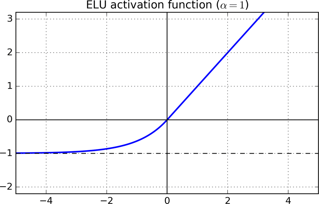

For the part x> 0, the gradient of ELU is 1, x
How to choose an activation function
Try ReLU activation first. Although we have listed some of the problems with ReLU above, many people have achieved good results using ReLU. According to the Occam's razor principle, it is better to try a simpler solution first. Compared with ReLU's powerful challengers, ReLU has the lightest computing power burden. If your project needs to be programmed from scratch, the implementation of ReLU is also particularly simple.
If ReLU does not work well, I will try Leaky ReLU or ELU again. I find that functions that can produce zero-centralized activation are generally much better than functions that cannot. ELU looks very attractive, but because the negative pre-activation value triggers a large number of exponential calculations, network training and inference based on ELU are very slow. If computing resources are not a problem for you, or the network is not particularly huge, choose ELU, otherwise, choose Leaky ReLU. Both LReLU and ELU add a hyperparameter that needs to be adjusted.
If the computing resources are abundant and the time is abundant, you can compare the performance of the above activation function with PReLU and random ReLU. If overfitting occurs, then random ReLU may be useful. Parametric ReLU adds a set of parameters that need to be learned. Therefore, parameterized ReLU should only be considered when there is a large amount of training data.
Concluding remarks
This article discusses what kind of data distribution is passed in, which is conducive to the proper learning of the neural network layer. The activation function implicitly normalizes these distributions, and a technique called Batch Normalization explicitly does this. Batch normalization is one of the major breakthroughs in the field of deep learning in recent years. However, we won’t discuss this technology until the next article in this series. For now, you can personally try to use different activation functions on your own network to see what effect! Happy experimenting!
Optical Fiber Patch Cord,Outdoor Ruggedized Patch Cords,Duplex Armoured Patch Cord,Indoor Patch Cord
ShenZhen JunJin Technology Co.,Ltd , https://www.jjtcl.com
